Introduction:
In the late 1980s, there was a lack of special analysis tools so, after that period, there was a rapid growth in developing the spatial data analysis software, particularly for the adoption and use of spatial statistics by Geographic Information Systems (GIS) researchers [1].
In the current world, we just can’t rely on mapping and visualizing the data. We have to convert those data into insights and have to move further by integrating statistical tools along with mapping tools for better visualization of both spatial and non-spatial data types. For that, the focus was given to different conceptual issues of integrating GIS and statistical tools.
And as a result, GeoDa, which consists of visualization, exploration, and explanation of interesting patterns in geographic data [1], has been developed.
What is GeoDa:
GeoDa, a user-friendly software program, and application evolved in 2003 with a view to help by providing free and open-source spatial analysis research infrastructure. It has one goal: To support researchers and analysts to meet the data-to-value issue. This issue entails translating records into insights.
![]()
Figure 1: GeoDa Icon
The application is designed for location-based data which include buildings, companies, or ailment incidents on the address level or aggregated to regions along with neighbourhoods, districts, or health regions. It has the main objective to provide a natural path to the user by an empirical spatial data analysis exercise from mapping to geo-visualization and exploration etc.
Also Read: GEODA: AN INTRODUCTION TO SPATIAL DATA ANALYSIS
History of Developing GeoDa:
GeoDa was developed and resealed in 2002 as separate software but before that, it was named DynESDA (Exploratory Spatial Data Analysis) which was used to work in ArcView 3.x [2] but developing this GeoDa has its history. When there was a need for integrating the statistical tools with mapping software, researchers started to think about the techniques for giving fruitful results and their framework.
In 1999 CSISS, a research infrastructure project funded by the U.S. National Science Foundation was founded to promote the spatial analytical study. It was quickly recognized that an easy-to-use, visual, interactive software package for non-GIS users would be an important tool in popularizing and facilitating spatial data analysis and would require as little other software as possible.
This is how GeoDa has been developed as the outcome of these problems.
Use of GeoDa:
GeoDa majorly helps to transform the data into insights that is adding statistical data and visualize by maps made. Its helps to enable to view the real time exploration of spatial data along with statistical data and observe the pattern of occurrence of a parameter.
By help of spatial statistical tests we can differentiate the actual spatial clusters from the clusters which just look like spatial cluster. Basically, real and non-real clusters can be differentiated. GeoDa includes Local Indicators of Spatial Association (LISA) to distinguish between hot spots and cold spots.
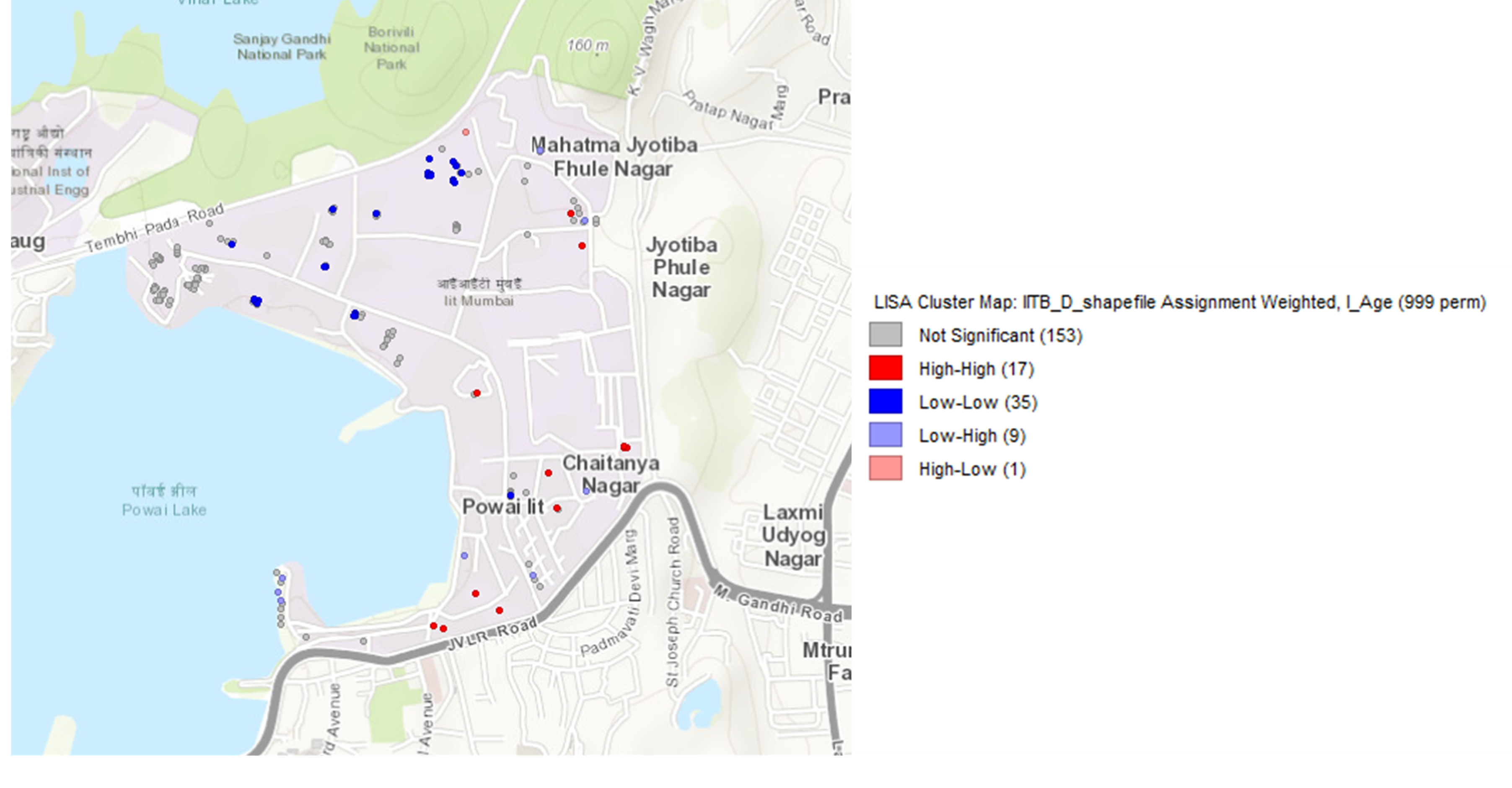
Figure 2: Detecting Hot Spots and Cold Spots by GeoDa
Source: [3]
An optimum amount of works can be done by the help of GeoDa in real life and that can be divided into 6 basic classes including –
- Spatial Data.
- Data Transforming.
- Mapping.
- EDA.
- Spatial Autocorrelation.
- Spatial Regression.
Table 1: Function of GeoDa
| Category | Functions |
|
Spatial data |
data input from shape file (point, polygon) |
| data input from text (to point or polygon shape) | |
| data output to text (data or shape file) | |
| create grid polygon shape file from text input | |
| centroid computation | |
| Thiessen polygons | |
| Data transformation | variable transformation (log, exp, etc.) |
| queries, dummy variables (regime variables) | |
| variable algebra (addition, multiplication, etc.) | |
| spatial lag variable construction | |
| rate calculation and rate smoothing | |
| data table join | |
| Mapping | generic quantile choropleth map |
| standard deviational map | |
| percentile map | |
| outlier map (box map) | |
| circular cartogram | |
| map movie | |
| conditional maps | |
| smoothed rate map (EB, spatial smoother) | |
| excess rate map (standardized mortality rate, SMR) | |
| EDA | histogram |
| box plot | |
| scatter plot | |
| parallel coordinate plot | |
| three-dimensional scatter plot | |
| conditional plot (histogram, box plot, scatter plot) | |
| Spatial Autocorrelation | spatial weights creation (rook, queen, distance, k-nearest) |
| higher order spatial weights | |
| spatial weights characteristics (connectedness histogram) | |
| Moran scatter plot with inference bivariate Moran scatter plot with inference | |
| Moran scatter plot for rates (EB standardization) | |
| Local Moran significance map | |
| Local Moran cluster map | |
| bivariate Local Moran | |
| Local Moran for rates (EB standardization) | |
| Spatial Regression | OLS with diagnostics (e.g., LM test, Motan’s I) |
| Maximum likelihood spatial lag model | |
| Maximum likelihood spatial error model | |
| predicted value map | |
| residual map |
Source: [1]
Planners also can use GeoDa for visualising the data and understand the statistical data in the space as well. It will help planners to maintain the proper track of their study. Urban planners mainly work in 4 major parts –
- Mapping and Geo-visualization.
- Multivariate EDA.
- Spatial Autocorrelation Analysis.
- Spatial Regression.
Mapping and Geo-visualization:
This can be done by collection of specialized choropleth maps, focused on highlighting outliers in the data. GeoDa helps to make cartogram, map animation in the form of a map movie, and conditional maps.
GeoDa helps to also visualize the significant and non-significant data and understand 4 types of a data that are –
- High – High: If Y increases then lagY also increases.
- High – Low: If Y increases then lagY decreases.
- Low – High: If Y decreases then lagY increases.
- Low – Low: If Y decreases then lagY also decreases.
Significance map shows the significance level of the significant data and Moran’s I shows the auto correlation among 2 variables.
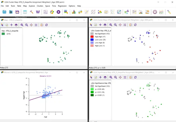
Figure 3: Basic Demonstration of GeoDa
Source: [3]
Multivariate EDA:
Multivariate exploratory data analysis is implemented in GeoDa through linking and brushing between a collection of statistical graphs [1]. These include the usual histogram, box plot, and scatter plot, but also a parallel coordinate plot (PCP) and three-dimensional scatter plot, as well as conditional plots (conditional histogram, box plot, and scatter plot).
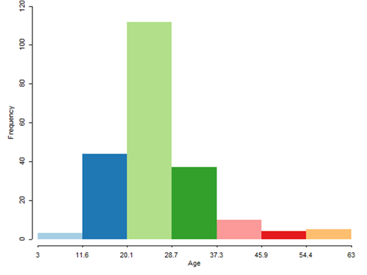
Figure 4: Histogram by GeoDa
Source: [3]
A histogram shows the organized grouped dataset of a particular range. Here age group 20.1 – 28.7 years has the maximum observations in the dataset.
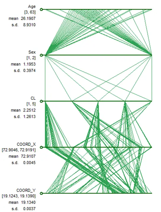
Figure 5: Parallel Coordinate Plot (PCP)
Source: [3]
This shows the relation between 5 parameters and how the pattern is that age, sex, K-means clusters, and X and Y coordinate of occurrence. So, we can refer that most of the cases in boy are near the age of 20 – 30 and ends at 63 whereas infection in girls starts at an earlier age. All the age group has been segregated into 5 clusters and most of the X-coordinates are near 72.90 with SD 0.0045 and most Y-coordinates are near 19.1390 with SD 0.0037.
Spatial Autocorrelation Analysis:
This is basically the test of Moran’s I either done by global method or local method.
- In global method slope of regression line resembles to Moran’s I. The traditional univariate Moran scatter plot has been protracted to represent bivariate spatial autocorrelation as well, that is, the correlation between one variable at a location, and a different variable at the neighbouring locations.
- Local analysis is based on the Local Moran statistic visualized in the form of significance and cluster maps [4].
If we see figure 3, then we can say that –
- Univariate Local Moran’s I show the occurrence of autocorrelation. Here due 153 observations are not significant but High-high and low-low autocorrelation have 17 and 35. So those are the points where the most significant dataset is there.
- With the continuation of the cluster map from Univariate Local Moran’s I, the significance map shows P = 0.05 with 45 observations and 0.001 with 1 observation. So, for 999 permutations 0.001 is the smallest p-value that shows the type of significance of the data.
- So, most of the data lie between -1 and +1so that part is most significant in the dataset.
Spatial Regression:
GeoDa also comprises a restricted degree of spatial regression functionality [5]. The simple diagnostics for spatial autocorrelation, heteroskedasticity and nonnormality, are applied for the standard ordinary least-squares regression. Estimation of the spatial lag and spatial error models is supported by means of the maximum likelihood (ML) method.
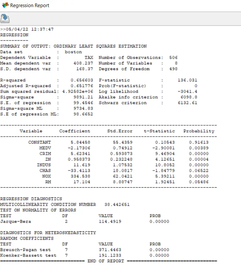
Figure 6: Regression Report by GeoDa
Source: [3]
- Akaike info criterion: The Akaike information criterion (AIC) is an estimator of prediction error and thereby relative quality of statistical models for a given set of data. Given a collection of models for the data, AIC estimates the quality of each model, relative to each of the other models. Thus, AIC provides a means for model selection.
- Breusch-Pagan test: In statistics, the Breusch–Pagan test, developed in 1979 by Trevor Breusch and Adrian Pagan, is used to test for heteroskedasticity in a linear regression model. It was independently suggested with some extension by R.
- Log Likelihood: The log-likelihood value of a regression model is a way to measure the goodness of fit for a model. The higher the value of the log-likelihood, the better a model fits a dataset. The log-likelihood value for a given model can range from negative infinity to positive infinity.
GeoDa V/S Other Similar Software:
What differentiates GeoDa from other data analysis tools is its focus on explicitly spatial methods for these spatial data.
We cannot directly compare GeoDa with other software, but we can come to a conclusion by seeing the applicability of it that, GeoDa is a combination of GIS and SPSS or other similar statistical tools as GeoDa do statistical analysis and shows the map for visualisation of data.
Features of GeoDa:
- GeoDa is a interface for Exploratory Spatial Data Analysis (ESDA) including spatial auto correlation (Moran’s I) for aggregating the data and find out the spatial regression.
- Different file formats can be supported including shapefile, KML, XLS (or CSV) kind tables, GeoJSON etc.
- Run in different operating system including Windows, Mac OS X, Linux etc.
- It is coded with help of C++.
Also Read: GeoDa – Exploratory Data Analysis and Spatial Regression
FAQs:
1. Why use GeoDa?
A user-friendly software program and free and open-source spatial analysis research infrastructure.
2. What is spatial data science?
Spatial data science (SDS) is a subset of Data Science that makes a specialty of the precise traits of spatial information, transferring past surely searching at in which matters occur to apprehend why they occur there.
3. What is spatial regression?
Spatial regression models, generally with a linear additive specification, wherein the connection amongst areal devices is detailed exogenously the usage of a weight matrix that mimics the spatial shape and the spatial interplay pattern.
4. Who developed GeoDa?
Luc Anselin.
5. What is spatial autocorrelation?
Spatial autocorrelation is the time period used to explain the presence of systematic spatial variant in a variable and nice spatial autocorrelation, that is most customarily encountered in sensible situations, is the tendency for regions or webweb sites which might be near collectively to have comparable values.
6. Why will we do spatial regression?
Regression (and prediction extra generally) offers us an ideal case to observe how spatial shape can assist us apprehend and examine our data.
Conclusion:
GeoDa-Web is a user-friendly cloud-to-cloud solution that provides price to present analytics structures through integrating web-based mapping with spatial analytics in an interactive exploratory framework. It flexibly integrates facts, spatial evaluation, cloud mapping and social community APIs to permit for the evaluation of large facts thru a number of devices [5].
Future improvement of the software program need to beautify this functionality and it’s miles was hoping that the pass to an open supply surroundings will contain an worldwide network of like-minded developers on this venture [1].
References:
- L. Anselin, Y. Kho and I. Syabri, “GeoDa: An Introduction to Spatial Data Analysis,” Geographical Analysis, vol. 38, pp. 5 – 22, 2006.
- “GeoDa,” Wikipedia, 2022. [Online]. Available: https://en.wikipedia.org/wiki/GeoDa.
- Author, 2022.
- L. Anselin, “Local Indicators of Spatial Association—LISA,” Geographical Analysis, vol. 27, pp. 93 – 115, 1995.
- L. Anselin, X. Li and J. Koschinsky, “GeoDa web: enhancing web-based mapping with spatial analytics,” in 23rd SIGSPATIAL International Conference, 2015.