Population Projection forms an integral part of any study or activity dealing with providing services to people. Planning for existing population can be done by obtaining population data from various sources. Meeting the future demand and upgrading the infrastructure requires insight about the population growth. If planning needs to be done for a new area then also projections are important for budgeting and upgrading purpose. Different types of Population projection methods are available to project the population depending on the nature and characteristic of an area. Some areas might be prone to large population increase due to in-migration whereas some areas might see increase in population due to natural growth or increased job opportunities. Various population projection methods have been described below in this article.
Related: Population projection | Meaning, Importance and Need

Mathematical and Graphical Methods
These are simple or direct methods since they operate with past population records and take no account of the components of change. Although the two types are somewhat interchangeable because mathematical methods can be plotted and graphical data can be described mathematically. Both methods are generally based on an idealized model of exponential growth followed by linear growth and finally decreasing growth.
These include:
- Linear growth
- Exponential growth
- Decreasing growth
- Correlation method
- Component method
Linear growth Method
Steady growth can be represented as:
DP / Dt = (Pb – Po) / (tb – to) = K1
where:
DP = change in population
Dt = change in time
Pb = base population (start of projection)
Po = initial population (in the applicable linear growth period)
tb = base year (start of projection)
to = initial year (earliest year in the applicable linear growth period)
K1 = growth rate = slope of line
A projection assuming linear growth can be calculated using the formula:
Pf = Pb + K1t
where:
Pf = future population
t = tf – tb = # of years projected into the future
tf = future year (end of projection)
Exponential growth
First-order growth can be represented as:
DP / Dt = K2P, or ln (Pb / Po) = K2(tb – to)
where:
DP = change in population
Dt = change in time
K2 = growth coefficient
P = population at a given year
Pb = base population (start of projection)
Po = initial population (in the applicable exponential growth period)
tb = base year (start of projection)
to = initial year (earliest year in the applicable exponential growth period)
A projection assuming exponential, or geometric, growth can be calculated using the formula:
Pf = PbeK2t
where:
Pf = future population
K2 = ln (Pb / Po) / (tb – to)
t = tf – tb = # of years projected into the future
tf = future year (end of projection)
Decreasing growth
Decelerating growth is assumed to asymptotically approach a saturation population, that is, the maximum population predicted for the geographic area of interest. The saturation population may be based on practical limitations such as the maximum number of dwellings under the zoning restrictions or other constraints.
Decreasing growth can be represented as:
DP / Dt = K3(S – P)
where:
DP = change in population
Dt = change in time
K3 = growth coefficient
S = saturation population
P = population at a given year
As P approaches S, DP / Dt approaches zero, and a projection assuming decreasing growth can be calculated using the formula:
Pf = S – (S – Pb)e-K3t
where:
Pf = future population
Pb = base population (start of projection)
K3 = -ln [(S – Pb) / (S – Po)] / (tb – to)
Po = initial population (in the applicable decelerating growth period)
t = tf – tb = # of years projected into the future
tf = future year (end of projection)
tb = base year (start of projection)
to = initial year (earliest year in the applicable decelerating growth period)
Correlation method
The correlation method uses a separate population projection for a similar community or region as a basis for determining a growth rate for the community or region of interest, assuming that the ratio of base populations is representative of the ratio of the projected populations. This method can be expressed mathematically as:
Pf2 / Pf1 = Pb2 / Pb1 = K4
where:
Pf2 = future population of community 2
Pf1 = future population of community 1
Pb2 = base population of community 2
Pb1 = base population of community 1
K4 = population ratio
Component method
This method, as suggested by its name, involves a summation of population growth components such as:
- Births
- Deaths
- Migration
- Employment opportunities
- Available housing
- Other data reflecting potential changes in the population
While this method may require significantly more effort than the previous methods, due to the amount of data needed, it may result in a more accurate projection if the data is accurate.
The component method can be represented by the following formula:
Pf = Pb + (F1 + F2 + … Fn)
where:
Pf = future population
Pb = base population
F1, F2, Fn = population changes expected during the selected time period due to specific factors (births, deaths, etc.)
While the above techniques may utilize plots of data, they are based on mathematical approaches. A purely graphical technique that could be called the superposition method may also be used. It involves an approach described below.
The Employment Method
Given a series of past values of the activity rate, i.e., economically active population / persons in working age groups = E / W
And the ratio, Persons in working age groups / total population = W / P
It is possible by using graphical or mathematical methods such as those just described to produce future values for these ratios. Then, given forecasts of total employment, population may be estimated, since
E/W X W/P = E/P
A range or employment forecasts (made for different assumptions about the economic ‘climate’) will yield a range of population forecasts. If regression techniques are used to project E/W and W/P, then the application of calculated estimating errors will of itself produce ranges of values for E/P. The reliability of this method is certainly no greater than those already discussed and should not be used for long-range forecasting.
Ratio Methods
This family of methods rests on the assumption that changes in any geographical area are a function of those experienced in (successively) wider areas. Thus, the population of a city is held to be a function of that of the region, which itself is a function of that of the nation, and so on.
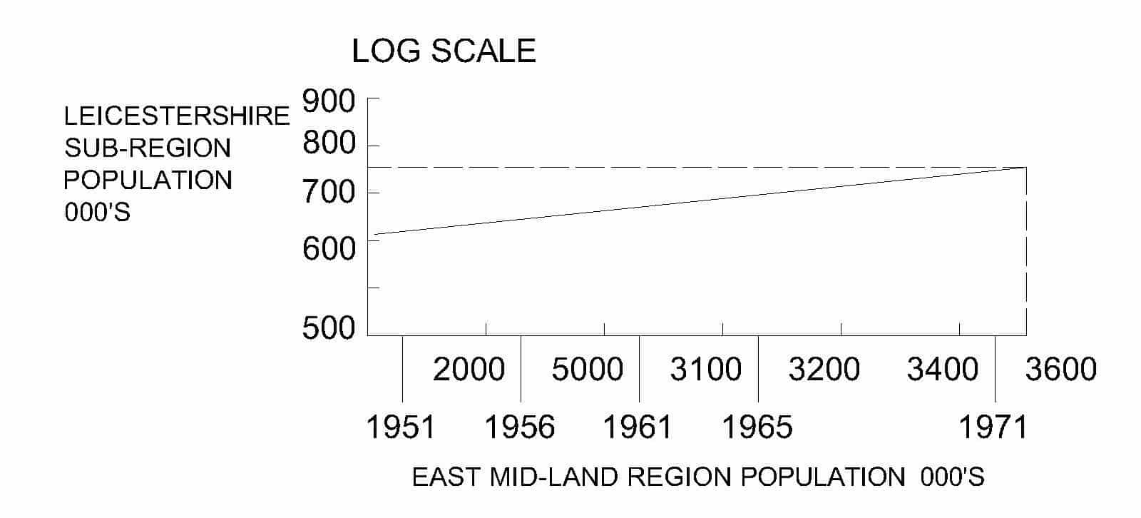
The requirements for such projections are time-series of populations for the areas to be used in the analysis and a forecast or set of forecasts for the largest area. In ratio methods the population of the second is plotted against that of the parent area (the nation), thus:
A curve is fitted to the points thus obtained and, by least squares, correlation, graphical or other method is extrapolated to intersect the projected value for the parent area at a given forecast date. Clearly, if a range had been given for the parent-area forecast this would have resulted in a range for the region.
In the second step down the process is repeated using data for the study area and the region.
Again the curve is fitted and extrapolated to intersect the (derived) forecast for the parent area.
This method has the great benefits of simplicity and the use of readily available data. However, this does not directly examine the components of population change which are subsumed in the central assumption, i.e. that there are certain forces at work in nations, regions and sub-regions which make for patterns and order in the proportionate share which the latter have in the former. Further, it is assumed that these relationships change but slowly over time.
The Migration and Natural Increase Method
This is the first method we have discussed in which an element of analysis occurs and as it name implies, the method enables natural and migratory changes to be handled separately.
By examining past data on net migration rates and by attempting to relate these to economic conditions, particularly to the demand for employment in the study area, it will be possible to adopt varying assumptions about the patterns of future migration. These might simply be ‘high’ and ‘low’ e.g. +5000 persons per annum and +1000 respectively; they may be expressed as different programmes e.g. +1000 per annum in the first 5 years, +2000 per annum in the following three years and +3000 per annum in the final 12 years (of a 20-year projection) would be programme 1. Other programmes would be developed which reflected as far as possible different assumptions about the size and timing of new job opportunities, housing land capacities, the output of the construction industry, the expansion of utilities and so on.

Next a set of programmes of future natural change would be developed either by subjective projection of past maximum and minimum rates or by ‘stepping down’ fro projections produced nationally or regionally. Of course, in some cases, projected natural changes might be available for the study area itself.
The essence of the method is to begin with the starting data population, add the net migratory element to produce the next figures to which is then added the natural change thus completing one cycle of the projection. The cycle may be for 1 year, 2 years, 5 years or other convenient period. The process is then repeated until the end of the projection period. Separate exercises are carried out for each set of natural change and migration assumptions.
Several points must be noted. Whilst this method is likely to be more accurate then the crude and simple methods so far discussed there are nevertheless a number of imperfections which limit its usefulness. First, the method uses total populations; age/sex structure is not accounted for. This means that changes in birth and death rates (the elements of natural change) which might result from changing age/sex structure cannot be seen and acted upon. Nor, of course, does the planner have the direct benefit of knowing this information for future times when estimating school-age population numbers of women of working age, etc. Whilst recognizing its great shortcoming, the migration and natural increase method does reveal the possible sequence and the main elements of change far better than the methods previously outlined. At the same time it is scarcely more time-consuming or expensive.
The Cohort-Survival Method
This is the standard method of population projection used by official (government) agencies in most advanced countries. It is not a rigid method, and can be adapted in a great variety of ways to suit the data available or the needs of the analyst whilst at the same time retaining its underlying logic.
The general form of the cohort-survival method is as follows. Males and females by single-year age groups are tabulated separately, the figures being extracted from the latest available census. Next the net migratory change for the first year is allowed for be the addition (or subtraction) of the assumed change for each age-group of males and females. Then the appropriate age-specific birth rates are applied successively to each group of women in the child-bearing range (usually 15-49 last birthday); the resultant births are divided into males and females, adjusted for mortality in the first year and entered in the next column, first row of the male female tables. Finally, age specific mortality rates of or survival rates are applied to each age-group of males and females to estimate the numbers who will survive to the next year (i.e. of their life and of the projection).
This sequence is repeated until the projection data is reached.
A very common simplification is to work with five-year (quinary) age groups 0-4, 5-9, 10-14,…etc. and to project by quinquennial periods, whilst possibly reducing the accuracy of the method and the degree of control which can be exercised over the process, the gains in time and the reduction of tedium (if manual calculation is used) may be felt o outweigh the losses. Slightly different data are needed e.g. five year fertility ratios to estimate births and, of course, the pattern of migration assumed must be expressed by five-year periods.
Population Projection method – Matrix Method
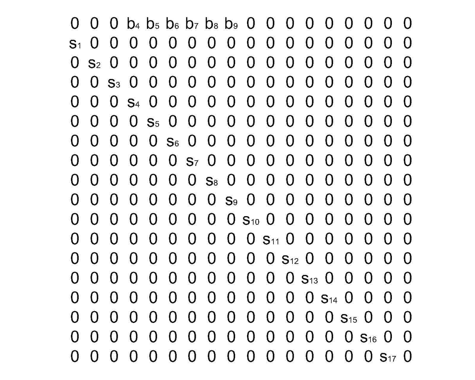
One of the latest and potentially most fruitful methods of population projection is to apply matrix algebra. Essentially, these methods follow the logic of the cohort-survival technique. The initial age-and-sex distribution is similarly represented as column sector but the incidence of births and deaths is handled by means of a ‘survivorship matrix’ which operates on the original population (column sector) to age the population through successive time periods, simultaneously performing the calculations of births and deaths. This matrix operator is of the form shown in Figure. The example given here is of for the female population grouped into quinary ranges of age (0-4, 5-9, 10-14, …85 and over). b4, b5,…..b10 are the age-specific birth rates and the sub-diagonal terms, s1, s2, s3, ….s17 the probabilities or survival from the nth to n+1th quinary age-range.
The effects of migration may be introduced by replacing the initial population vector by a matrix in which columns are regions or areas and where rows, as before, are the age groups. Similarly the survivorship matrix is replaced by a set of matrices, one for each region.
Migration is then introduced by means of a set of transition matrices (one for each age group) in which the elements represent the probability that an individual of that age group and in region i at any time will move to region j in the next time period.
The population projection is then carried out by multiplying the initial population matrix (columns are regions, rows are age-groups) by survivorship matrix and then adding the net migration matrix (whose rows are age groups and whose columns are regions).
The method is appealing in its elegance and yet leaves certain questions unanswered for example survival-and-birth-rates are assumed constant over time and over each age group. None of these assumptions could easily be defended in the majority of practical applications. Nevertheless, the method appears to have enormous potential, especially as it seems capable of handling interregional migrations, both inward and outward, and specific to age group and sex. It also seems capable of doing so with economy and elegance of operation in a manner ideally suited to simple computer operations.


